R Data Structure

Type Data Structure:

Data Structure can be defined as the specific form of organizing and storing the data. R Programming supports five basic types of data structure namely Vector, matrix, Array, , and list.

Vector:

Vector is a sequence of data elements of the same basic type. Members of a Vector are formally called components. Whenever we are storing the numerical value in ‘a’ or ‘b’ that ‘a’ or ‘b’ nothing but a Vector, so Vector is one-dimensional array used to store collection data of the same data type.

                                     

Similar kind of data type you can store like all the Numeric data(data type numeric) in a Vector, again you can store complex(data type complex) similarly in logical(data type logical)  or character(data type character) you can store this thing in a Vector. There is six type of atomic Vector, they are Logical, Integer, Double, Complex, Character, and Raw.

Matrices:

Matrix is a collection of data elements of the same mode arranged in a two-dimensional rectangular layout. We can create a matrix containing only characters or only logical values, these are not of much use. We use matrices containing numeric elements to be used in mathematical calculations. They are accessed by two integer indices.

Three kinds of matrices are

• Matrix Multiplication
• R matrix transpose
• Matrix power

Arrays:

Similar to matrices but they can be multi-dimensional(more than two dimensions). Array function() takes vectors as input and uses the values in the dim parameter to create an array.

If you want to store age, salary, location, designation then it becomes your array. Salary or age all those things are numeric but if you store numeric as well as a character variable, character variable is nothing but a gender like male or female then you can use an array.

Data Frames:

Generalization of matrices where different columns can store in a different mode then it’s called Data Frame. It is a list of vectors of equal length.  Data frame is a table or two-dimensional array like structure in which each column contains values of one variable and each row contains one set of values from each column. It can store a different kind of data types like you can store numerical with categorical and logical

Lists:

Lists are something where you can store all those other four, you can store data frame in lists, you can store an array in a list or you can store matrices and you can store a vector as well. Lists ordered a collection of objects where the elements can be of different types. Lists contain the elements of different types like-number, strings, vectors and another list inside it. Lists are created using lists function().

Types of Data Structure:

Vector, Matrix, and Array those are in the homogeneous so they can store homogeneous data either numeric, character or logical but only different in dimension, Vector is one dimension, Matrix is two dimension and Array is multidimensional. 

                  

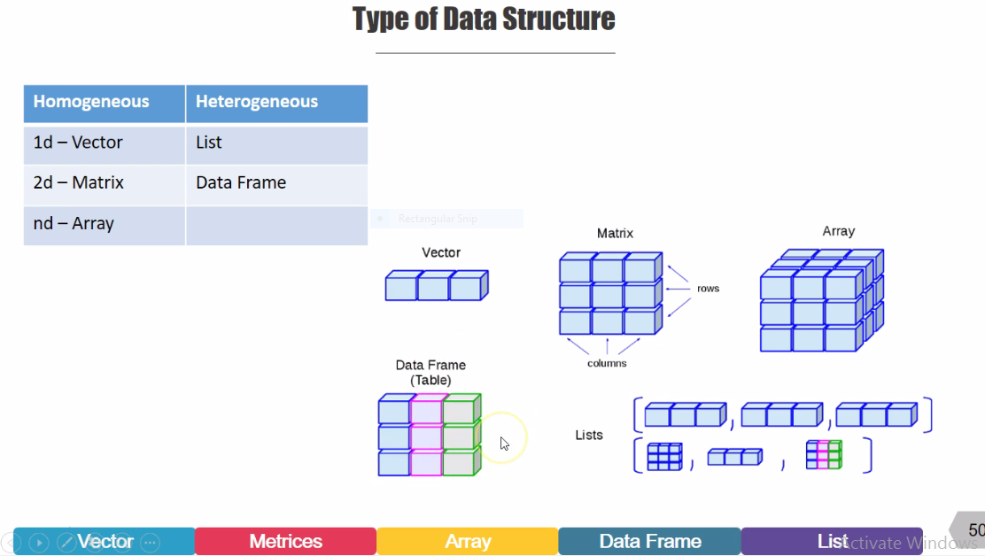
On the other side if you talk about Data frame and lists those are in heterogeneous so they can store a different kind of data type.

                                                                                  VECTOR

Numeric Vector:

Now we will learn about the Vector. Suppose you want to store 42 (vec1<-42)in vector 1 then you can see the result in vector 1. Similarly if you store more than variable 1-5 (vec1<-c(1,2,3,4,5) .  

            

Here we show you both the way either you can use combine function and use “,” and you can store 1,2,3,4,5  (vec1<-c(1,2,3,4,5) or you can store 1-5 (vec1<-c(1:5) the only advantage is suppose you want to store it 1,7,9,3,5 then also you can use the combine function and you can store it.

                  

                    

If you see the class of the vector 1 then it would be an integer. Likewise, if you want to access a particular suppose you have like 1,2,3,4,5  but you only access the second element of your vector then you would get probably 2 since 1-5 in store. Likewise, you can also access 1 and 3 from that vector

Character Vector:

Within double coat, you just pass the value which you want to store. Suppose in Vec2 we want to in “universe” (vec2<-”Universe” ) but if you store more than 1 character variable.      

    

Then you have to use the combine function (vec2<-c(“Universe”,”sun”,”moon”) and if you see the class of it then you definitely get the class as character.

If you mix the character and numeric then all the values will be converted to character.

Logical Vector:

You can store TRUE and FAlSE for the logical function. Suppose we are using vector 3. Here you store FALSE for vec3(Vec3<-FALSE). In vec3 if you store more than one variable which is TRUE and FALSE (Vec3<-c(TRUE, FALSE) and finally if you class of it, it would be logical. 

If you mix the logical vector function with numeric vector function then the numeric function gets the preferences and If you mix character with logical function and numeric function then all value converted to character function so character is given the preferences.

Matrices:

Matrices are the R object, which is a collection of data elements arranged in a two-dimensional data array.Although we can create a matrix containing only characters or only logic values which are not of much use. We use matrices containing numeric elements to be used in mathematical calculations.

Matrix is created using the matrix() function.Matrix() function is being used to create a matrix. Here we show an argument.

Here,the argument is matrix(data=NA,nrow=1,ncol=1,byrow=FALSE,dimnames=NULL). We have a data, word data which we want to create a matrix, suppose 1-4 we want to create a matrix. Then, how many rows here, there are by default 1 row but we are changing it two and by default it’s column is 1 but we are also changing this to two and suppose by default byrow is equal to False and by row is nothing but suppose 1-4 you want to create a matrix then how you want to do it? Either this way byrow equal to TRUE equal to 1,2,3 and 4. 

But if you change that byrow equal to FALSE then you want to do it by column so first 1 then 2 then 3 then 4 that’s how you can do it. Here, we are keeping all the numerical values but here we are showing it 2 rows and 2 columns and by rows equal to TRUE that means we will start from the row and then in the second row.  Similarly, if you access any element of a matrix.

 

Suppose, we are creating matrix 2 where we access the first row then you can say 1,so this is row, column so we are asking for the first row and it would give us first row, the second row then it also gave us first column because we said row, column then second column. 

We haven’t written anything in a row that’s why it would give us all the rows and only it would give us first column. Similarly, it would give us all the rows but an only second column.

Array:

Now we have discussed the Array. An Array is similar to matrices but it can have more than two dimensions. Here, you can store 2*3*4 anything you can create. R Array is the data objects which can store data in more than two dimensions. An Array is created using the Array() function. The array can store only data type. Array takes vectors as input and uses the values in the dim parameter to create an Array.

                  

 It can contain multidimensional rectangular shaped data storage structure. “Rectangular” in the word, each row is having the same length similarly for each column and other dimensions. But Array can store only values which have similar kind of data,i.e. variables/elements having a similar data type.We create Array using the Array() function. The argument is array (data=NA, dim=Length(data), dimnames=NULL). 

                  

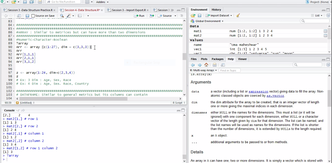
We first pass the data here we pass 1 to 27 with this dataset we want to create the Array. What is those dimension? The dimension is 3*3*3 here you can store salary, age, designation, grade or something like that. It is pretty simple and you can see the result as well.

Dataframe:

Dataframe is a table or two-dimensional array like structure where each column contains values of one variable and each row contains one set of values from each column.

Data frame is used for storing a data tables. This is a list of vectors of equal length. All the vectors we have learned previously like Numerical vectors, Character Vectors, Logical Vectors and all those things. Now you just mix them the three vectors you mix them. Suppose you want to create a data frame where you have one attribute as Numerical like age or salary which is numerical but you have three employees so all of this vector like the same length. So you have three employees then you want to store their gender as well male, female. Similarly, you want to understand whether they left the company or not something like that TRUE FALSE or something like that. If you achieve this kind of data set then you have to use data frame.

                 

Now we use data. frame, we use this data. frame function. Before that we have to three vectors first, suppose we are storing 2,3,5 a vector called num then “aa”,”bb”,”cc” in char and then TRUE, FALSE and TRUE in logical then ultimately using data.frame()function and creating that data frame. Here we are using the data frame name df. If you want to see what is df? Or what is being stored in df? Thereafter you get the result.

                 

Think about a business scenario, where you have a lot of employees and here you use the data frame. That’s why data frame is one of the most important structures in R. In R we have a lot of inbuilt data frame which you can explore. One of the popular dataframe is mtcars. Mtcars is a dataset of a car distribution. We have df which is already been created in R that’s why we said this inbuilt database. Here mtcars has 32 model of cars. If you want to see a couple of them then you use head() function, you can use the head() function for first several rows. similarly, you can use tail() function to see last couple rows. The tail function gives you the below of the lists. Another function is str() function which is the structure of a dataset.  The str() function gives you the detail observation. For str() function you get a sense how your data set looks like. Likewise, you can see the summary which is better than the full data structure. The summary() function gives you the min or max from each of those attributes.

Accessing Column from data frame:

Accessing Column from data frame is quite easy. Once you write any data frame and after that if you put “dollar sign ($)” then you would see all the columns whatever it contains and you can see whatever is there in that column.

Now, there is another way to do it, if you use “third bracket[]” and if you use row, column as I discussed earlier.

Similarly, you can name the column and you can see the column as well. But it has a problem if you have more than one column then how do you do that? In that case, you use combine function and give the number of all those columns and you can see those columns as well.

Accessing Row:

Similarly, Accessing Row is also easy. As said use third bracket and between third bracket row, column.

For an example: df[2,]

Here row value is 2 and all column value is NULL. The function is used for accessing the second row.

                       

Dropping column:

If you want to drop a column then you don’t want the column to be included in your data frame.You simply put (-sign) before that number. If you say that you don’t want to see drop third column which is actually displacement column.

For an example: df[,-3]

                          df[,-c(2,3)]

So if you say within third bracket all the rows,-3 then it would actually drop that column. Similarly, if you drop second and third then it would actually drop displacement and cylinder.

Subset:

The fourth one is a subset. So, what if you don’t want to see all the rows of that column. You want to see only those observation or those car brands where the cylinder value is more than 6 or the horsepower is more than 50.

For an instance: car 1<-subset (df,cyl>6)

       car 2<-subset (df,hp>50)

Then you create new data frame called car 1 using the subset function so in subset function you passing the data when you are passing the condition. Based on that your car is created, you can see it cylinder column of car data frame, has the only cylinder which is more than 6. Similarly, for horsepower also you can see the result.

                

If you have two data frame, so you have data frame one and data frame two now you have combined them by row. Suppose, in the first data frame you have twenty car brands and second data frame you have twelve car brands. Now you want to combine this two rbind () function.

                 

Likewise, if you have two columns. Suppose all the 32 car brands you have the mileage which is a column and you have another one may be a cylinder. So you want to combine this column that also you can do using cbind() function.

Factor:

In a data frame, character vectors are automatically converted into factors, and the number of levels can be determined as the number of different values in such a vector. You can create a data frame using more than one data types. It can be a mixture of numeric, with a character with logical all those things. 

              

Similarly, if you see the showing data frame which has three vectors like name, age and gender and you have created a new data frame using data.frame() function. If you see the class of it, you would get it as data.frame. But surprisingly if you see the class of name this data frame dollar could give all those names. If you see the class of it you would be surprised this is now not a character variable rather it’s now a factor. So it is another new data type.

Factor:

In a data frame, character variables are automatically changed or converted into factor, and the number of levels can be determined as the number of different values in such a vector.

Factor takes a limited number of different values, such variables are referred to as categorical variables. So, Factor represents the categorical data,  the factor can be ordered or unordered and are an important class for statistical analysis and for plotting. Factor variables are very useful to many different types of graphics.

Storing data factors insures that the modeling functions will treat such data correctly. The factor can store both integers and strings. These are very useful in the columns which have a limited number of unique values such as “Male, Female” and “True, False” etc.

Factors in R has two varieties

• ordered
• unordered.

Factors are stored as a vector of integer values, with a corresponding set of character values to use when the factor is shown. factor() function is used to create a factor. The required argument to factor is a vector of values, which will be returned as a vector of factor values. Numeric and Character variables both can be made into factors, but a factor’s levels will always be character values.

Factor levels

Getting a dataset you will look that it contains factors with specific factor levels. By the way, sometimes you will willing to change the names of these levels for clarity or any other reasons. R permits you to do this with the function levels().

Examples:

for this is mtcars data:

>Str (mtcars)

$ cyl : num 6 6 4 6 8 6 8 4 4 6

Here, have shown an example, suppose this is mtcars data where has 32 car brands. Each of those cars we have eleven attributes like horsepower, cylinder, displacement, mileage or all those things. If you see the cylinder, either it has 6 as cylinder or 4 as cylinder or 8 as a cylinder. So, since if you have a minimum number of unique value of particular attributes then that’s an ideal candidate for factors. Because it does not take 6.5 or 4.32 or 5.67. It takes either 4 or 6 or 8 so we want to change this to a factor.

Str (mtcars)

mtcars$cyl = as.factor(mtcars$cyl)

How to use factor() function? Just use as.factor() function, here the first query is which one you want to change? Suppose, here change the “mtcars$cylinder”.You can access it any column using the dollar function. Using that “as.factor()” function,the “mtcars$cylinder” is converting into Factor.

Str (mtcars)

$ cyl : num 6 6 4 6 8 6 8 4 4 6

Now, looking carefully at the above example, look the structure of “mtcars” when it changes to factor then everything is changed into the numeric function. Changing this when you look at the cylinder, it is converted to a factor. After changing it has three level 4,6 and 8.

str (mtcars)

(four column or four attributes change to numericals factors)

$ am : factor w/2 levels “0” , “1” : 2 2 2 1 1 1 1 1 1 1 . . .

If it is changed whether manually or automatically. What is the number of gear of the mtcars or how many numbers of carburetors is there, then you see the number of the structure of mtcars. Now you see all those columns or all those attributes as change into factor. You can notice that automation has two levels if it is manual or automatic.

                                      

str (mtcars)

(four column or four attributes change to numericals factors)

$ gear : factor w/3 levels “3” , “4” , “5”  : 2 2 2 1 1 1 1 2 2 2 . . .

You have three gears levels.

str (mtcars)

(four column or four attributes change to numericals factors)

$ carb: factor w/6 levels “1” , “2” , “3” , “4”,. . : 4 4 1 1 2 1 4 2 2 4. . .

Similarly, you have 6 levels of carbs. That’s how you can change it.

How to change the name of the level?

If you change the name of the level, then you have to create a new variable called gender vector and then you want to store “Male”, “Female” , “Female” , “Male” , “Male”. It may be a data for five employees. Thereafter, you see that the five things have been recorded. If you see the class of gender vector then it is a character vector.

gender vector <-c ( “Male”, “Female” , “Female” , “Male” , “Male” )

gender vector

class ( gender vector )

• But, if you want to change the gender vector to factor

#Convert gender vector to factor

factor-gender-vector <-as.factor(gender vector)

factor-gender-vector # factor gender has two levels Male and Female

then use “as.factor” and then see it has changed to a factor and it’s showing the level is “Female Male”.

Now you want to change the name of the factors using level()

levels(factor-gender-vector)<-c(“f” , “M”)

levels: Female and Male(earlier)

Now, it changes to “F & M”

That’s how you want to do it.

How to do that? In this case, level() function helps you. Using level() function which you want to change, just give this. Suppose you want to change “factor-gender and vector”. Here suppose you want to change F and M for Female and Male. once you can do it and you can again see this, this levels have changed. Previously it showed Female and Male now it changes to F and M. in this process you want to do it.

List:

These are the most complex data structure. A List may contain a combination of vectors, matrices, data frames and even other list itself. The list is being created using List() function in R.  A list is a generic vector containing other objects. Lists is a data structure containing of mixed data types. A vector which have all elements of same type is called atomic vector but a vector having elements of various type is called List.

                                                               

Before creating a list, creating a vector suppose you create a vector with one to ten(1-10).

Thereafter you create a matrix which is two dimensional array.

Then you will create a data frame, that is “mtcars” which was inbuilt data frame but here you just take only three observation and create a data frame called “my-dataframe” from “mtcars”.

Finally, you will store this vector, matrix and dataframe in a list called “my list”, using the list() function.

If you created the list() then you see the result. You can see the output from “mylist”. Here the list starts from the first vector,”my-vector” is one to ten.

Creating list:

# vector with numerics from 1 up to 10

>my-vector <-1:10

The output is

                                                             [[1]]

                                                             

Thereafter you create a matrix which is two dimensional array that “my-matrix”.

# matrix with numerics from 1 up to 9

>my-matrix <-matrix(1:9,ncol =3)

The output is

                                                              [[2]]

                                                                        

Then you just created the data frame

# first 3 rows of the built in data frame “mtcars”

>my-df <-mtcars [1:3,]

The result is

                                                              [[3]]  

                                 

        

That’s the way to do a list.

If you see these examples there's no name like [1], [2], and [3] is written of the list but you can change those name as well using the name() function.

#give name using name()

>names (my list)<-c (“vec”, ”mat”, ”df”)

Then you can check the output and see the name would be changed.

How does a list() work?

At first you create vector() function

my-vector<-1:10

Then use matrix function

my- matrix<-(matrix 1:9, ncol=3)

Thereafter creating a dataframe

my-df<-mtcars[1:3,]

Here”mtcars” is the data where you can see all those 32 car brands and eleven attributes but the first 3 rows uses for this dataframe.

Then using the list() function,created a list

my-list < - list(my-vector,my-matrix,my-df)

Then the output is  my-matrix ,my-vector, and my-df

                                                                  1.

                                                                      

                                                    2.

                                                         

                             3.

                                 

In this way list works.

List is the end of data structure. Any character variables when it goes to data frame it automatically changes to a factor but if you don’t want to do this then you can change that things from anything to anything. Here show you how to change anything to a factor using as.factor but later you also know where you will be change it to,as numeric() function or as character() function. 


mutate(),filter(),arrange() Function

Selecting columns using select()

select() keeps only the variables you mention

Use This Command To Perform The Above Mentioned Function

#######################################
#select(): Select specific column from tbl
#######################################
tbl <- select (hflights, ActualElapsedTime, AirTime, ArrDelay, DepDelay )
glimpse(tbl)

#starts_with("X"): every name that starts with "X",
#ends_with("X"): every name that ends with "X",
#contains("X"): every name that contains "X",
#matches("X"): every name that matches "X", where "X" can be a regular expression,
#num_range("x", 1:5): the variables named x01, x02, x03, x04 and x05,
#one_of(x): every name that appears in x, which should be a character vector.

#Example: print out only the UniqueCarrier, FlightNum, TailNum, Cancelled, and CancellationCode columns of hflights

select(hflights, ends_with("Num"))
select(hflights, starts_with("Cancel"))
select(hflights, UniqueCarrier, ends_with("Num"), starts_with("Cancel"))

Create new columns using mutate()

mutate() is the second of five data manipulation functions you will get familiar with in this course. mutate() creates new columns which are added to a copy of the dataset.

Use This Command To Perform The Above Mentioned Function

#######################################
#mutate():  Add columns from existing data
#######################################
g2 <- mutate(hflights, loss = ArrDelay - DepDelay)
g2

g1 <- mutate(hflights, ActualGroundTime = ActualElapsedTime - AirTime)
g1

#hflights$ActualGroundTime <- hflights$ActualElapsedTime - hflights$AirTime

#######################################

Selecting rows using filter()

Filtering data is one of the very basic operation when you work with data. You want to remove a part of the data that is invalid or simply you’re not interested in. Or, you want to zero in on a particular part of the data you want to know more about. Of course, dplyr has ’filter()’ function to do such filtering, but there is even more. With dplyr you can do the kind of filtering, which could be hard to perform or complicated to construct with tools like SQL and traditional BI tools, in such a simple and more intuitive way.

R comes with a set of logical operators that you can use inside filter():
• <
• <=
• == 
• !=
• !=
• > 

Use This Command To Perform The Above Mentioned Function

#filter() : Filter specific rows which matches the logical condition
#######################################
#R comes with a set of logical operators that you can use inside filter():

#x < y, TRUE if x is less than y
#x <= y, TRUE if x is less than or equal to y
#x == y, TRUE if x equals y
#x != y, TRUE if x does not equal y
#x >= y, TRUE if x is greater than or equal to y
#x > y, TRUE if x is greater than y
#x %in% c(a, b, c), TRUE if x is in the vector c(a, b, c)

# All flights that traveled 3000 miles or more
long_flight <- filter(hflights, Distance >= 3000)
View(long_flight)
glimpse(long_flight)

# All flights where taxing took longer than flying
long_journey <- filter(hflights, TaxiIn + TaxiOut > AirTime)
View(long_journey)

# All flights that departed before 5am or arrived after 10pm
All_Day_Journey <- filter(hflights, DepTime < 500 | ArrTime > 2200)

# All flights that departed late but arrived ahead of schedule
Early_Flight <- filter(hflights, DepDelay > 0, ArrDelay < 0)
glimpse(Early_Flight)

# All flights that were cancelled after being delayed
Cancelled_Delay <- filter(hflights, Cancelled == 1, DepDelay > 0)

#How many weekend flights flew a distance of more than 1000 miles but 
#had a total taxiing time below 15 minutes?

w <- filter(hflights, DayOfWeek == 6 |DayOfWeek == 7, Distance >1000, TaxiIn + TaxiOut <15)
nrow(w)

y <- filter(hflights, DayOfWeek %in% c(6,7), Distance > 1000, TaxiIn + TaxiOut < 15)
nrow(y)

#######################################

Arrange or re-order rows using arrange()

To arrange (or re-order) rows by a particular column such as the taxonomic order, list the name of the column you want to arrange the rows 

Use This Command To Perform The Above Mentioned Function

#######################################
#arrange(): reorders the rows according to single or multiple variables,
#######################################
dtc <- filter(hflights, Cancelled == 1, !is.na(DepDelay)) #Delay not equal to NA
glimpse(dtc)

# Arrange dtc by departure delays
d <- arrange(dtc, DepDelay)

# Arrange dtc so that cancellation reasons are grouped
c <- arrange(dtc,CancellationCode )

#By default, arrange() arranges the rows from smallest to largest. 
#Rows with the smallest value of the variable will appear at the top of the data set. 
#You can reverse this behavior with the desc() function. 

# Arrange according to carrier and decreasing departure delays
des_Flight <- arrange(hflights, desc(DepDelay))

# Arrange flights by total delay (normal order).
arrange(hflights, ArrDelay + DepDelay)

#######################################

The summarise() function will create summary statistics for a given column in the data frame such as finding the mean.

Use This Command To Perform The Above Mentioned Function

#######################################
#summarise(): reduces each group to a single row by calculating aggregate measures.
#######################################
#summarise(), follows the same syntax as mutate(), 
#but the resulting dataset consists of a single row instead of an entire new column in the case of mutate()

#min(x) - minimum value of vector x.
#max(x) - maximum value of vector x.
#mean(x) - mean value of vector x.
#median(x) - median value of vector x.
#quantile(x, p) - pth quantile of vector x.
#sd(x) - standard deviation of vector x.
#var(x) - variance of vector x.
#IQR(x) - Inter Quartile Range (IQR) of vector x.
#diff(range(x)) - total range of vector x.

# Print out a summary with variables 
# min_dist, the shortest distance flown, and max_dist, the longest distance flown
summarise(hflights, max_dist = max(Distance),min_dist = min(Distance))

# Print out a summary of hflights with max_div: the longest Distance for diverted flights.
# Print out a summary with variable max_div
div <- filter(hflights, Diverted ==1 )
summarise(div, max_div = max(Distance))

summarise(filter(hflights, Diverted == 1), max_div = max(Distance))

###########################################################

Pipe operator: %>%

Before we go any futher, let’s introduce the pipe operator: %>%. dplyr imports this operator from another package (magrittr). This operator allows you to pipe the output from one function to the input of another function. Instead of nesting functions (reading from the inside to the outside), the idea of of piping is to read the functions from left to right.

Use This Command To Perform The Above Mentioned Function

#######################################
#Chaining function using Pipe Operators
#######################################
hflights %>%
  filter(DepDelay>240) %>%
  mutate(TaxingTime = TaxiIn + TaxiOut) %>%
  arrange(TaxingTime)%>%
  select(TailNum )

# Write the 'piped' version of the English sentences.
# Use dplyr functions and the pipe operator to transform the following English sentences into R code:

# Take the hflights data set and then ...
# Add a variable named diff that is the result of subtracting TaxiIn from TaxiOut, and then ...
# Pick all of the rows whose diff value does not equal NA, and then ...
# Summarise the data set with a value named avg that is the mean diff value.

hflights %>%
  mutate(diff = TaxiOut - TaxiIn) %>%
  filter(!is.na(diff)) %>%
  summarise(avg = mean(diff))

# mutate() the hflights dataset and add two variables:
# RealTime: the actual elapsed time plus 100 minutes (for the overhead that flying involves) and
# mph: calculated as Distance / RealTime * 60, then
# filter() to keep observations that have an mph that is not NA and that is below 70, finally
# summarise() the result by creating four summary variables:
# n_less, the number of observations,
# n_dest, the number of destinations,
# min_dist, the minimum distance and
# max_dist, the maximum distance.

# Chain together mutate(), filter() and summarise()
hflights %>%
  mutate(RealTime = ActualElapsedTime + 100, mph = Distance / RealTime * 60) %>%
  filter(!is.na(mph), mph < 70) %>%
  summarise(n_less = n(), 
            n_dest = n_distinct(Dest), 
            min_dist = min(Distance), 
            max_dist = max(Distance))

#######################################

Group operations using group_by()

The group_by() verb is an important function in dplyr. As we mentioned before it’s related to concept of “split-apply-combine”. We literally want to split the data frame by some variable (e.g. taxonomic order), apply a function to the individual data frames and then combine the output.

Use This Command To Perform The Above Mentioned Function

#######################################

#group_by function 

#######################################

# Most data operations are done on groups defined by variables.

# group_by() takes an existing tbl and converts it into a grouped tbl where operations are performed "by group".

# Make an ordered per-carrier summary of hflights

hflights %>%

  group_by(UniqueCarrier) %>%

  summarise(p_canc = mean(Cancelled == 1)*100,

            avg_delay = mean(ArrDelay,na.rm = TRUE))%>%

  arrange(avg_delay, p_canc)

# summary of hflights without per carrier

hflights %>%

  summarise(p_canc = mean(Cancelled == 1)*100,

            avg_delay = mean(ArrDelay,na.rm = TRUE))%>%

  arrange(avg_delay, p_canc)

# Ordered overview of average arrival delays per carrier

# mutate() uses the rank() function, that calculates within-group rankings.

# rank() takes a group of values and calculates the rank of each value within the group,

hflights %>%

  filter(!is.na(ArrDelay), ArrDelay>0) %>%

  group_by(UniqueCarrier) %>%

  summarise (avg = mean(ArrDelay))%>%

  mutate(rank = rank(avg)) %>%

  arrange(rank)

####################################################################################

####################################################################################

Date with R

Dates can be imported from character, numeric formats using the as.Date function from the base package.

If your data were exported from Excel, they will possibly be in numeric format. Otherwise, they will most likely be stored in character format. If your dates are stored as characters, you simply need to provide as.Date with your vector of dates and the format they are currently stored in

There are a number of different formats you can specify, here are a few of them:

%Y: 4-digit year (1982)

%y: 2-digit year (82)

%m: 2-digit month (01)

%d: 2-digit day of the month (13)

%A: weekday (Wednesday)

%a: abbreviated weekday (Wed)

%B: month (January)

%b: abbreviated month (Jan)

Use This Command To Perform The Above Mentioned Function

####################################################################################

####################################################################################

# Lesson 6:

# Topic 3: Date in R

###################################################################################

# Today's date

today <- Sys.Date()

today

class(today)

#Creating date from character

character_date <- "1957-03-04"

class(character_date)

# Convert into date class by as.Date function

sp500_birthday <- as.Date(character_date)

sp500_birthday

class(sp500_birthday)

# Date format

#default - ISO 8601 ISO 8601 Standard: year-month-day

as.Date("2017-01-28")

# Alternative form: year/month/day

as.Date("2017/01/28")

#Fails: month/day/year

as.Date("01/28/2017")

# Explicitly tell R the format

as.Date("01/28/2017", format = "%m/%d/%Y")

#Date format

# %d - Day of the month (01-31)

# %m - Month (01-12)

# %y - Year without century (00-99)

# %Y - Year with century (0-9999)

# %b - Abbreviated month name

# %B - Full month name

# "/" "-" "," Common separators

# Example: September 15, 2008

as.Date("September 15, 2008", format = "%B %d, %Y")

# Extract the Weekdays

dates <- as.Date(c("2017-01-02", "2017-05-03", "2017-08-04", "2017-10-17"))

dates

weekdays(dates)

# Extract the months

months(dates)

# Extract the quarters

quarters(dates)