In the past few years, video analytics, also known as video content analysis or intelligent video analytics, has attracted increasing interest from both industry and the academic world. Thanks to the enormous advances made in deep learning, video analytics has introduced the automation of tasks that were once the exclusive purview of humans.
Recent improvements in video analytics have been a game-changer, ranging from applications that count people at events, to automatic license plate recognition, along with other more well-known scenarios such as facial recognition or smart parking.
CCTV surveillance camera detecting vehicles in real-time in order to recognize specific events, such as car accidents, and trigger alerts accordingly.
Image source
This kind of technology looks great, but how does it work and how can it benefit your business?
In this guide, you’ll discover the basic concept of video analytics, how it’s used in the real world to automate processes and gain valuable insights, and what you should consider when implementing an intelligent video analytics solutions in your organization.
What is intelligent video analytics?
The main goal of video analytics is to automatically recognize temporal and spatial events in videos. A person who moves suspiciously, traffic signs that are not obeyed, the sudden appearance of flames and smoke; these are just a few examples of what a video analytics solution can detect.
Real-time video analytics and video mining
Usually, these systems perform real-time monitoring in which objects, object attributes, movement patterns, or behavior related to the monitored environment are detected. However, video analytics can also be used to analyze historical data to mine insights. This forensic analysis task can detect trends and patterns that answer business questions such as:
When is customer presence at its peak in my store and what is their age distribution?
How many times is a red light run, and what are the specific license plates of the vehicles doing it?
Some known applications
Some applications in the field of video analytics are widely known to the general public. One such example is video surveillance, a task that has existed for approximately 50 years. In principle, the idea is simple: install cameras strategically to allow human operators to control what happens in a room, area, or public space.
In practice, however, it is a task that is far from simple. An operator is usually responsible for more than one camera and, as several studies have shown, upping the number of cameras to be monitored adversely affects the operator’s performance. In other words, even if a large amount of hardware is available and generating signals, a bottleneck is formed when it is time to process those signals due to human limitations.
Video analysis software can contribute in a major way by providing a means of accurately dealing with volumes of information.
Video analytics with deep learning
Machine learning and, in particular, the spectacular development of deep learning approaches, has revolutionized video analytics.
The use of Deep Neural Networks (DNNs) has made it possible to train video analysis systems that mimic human behavior, resulting in a paradigm shift. It started with systems based on classic computer vision techniques (e.g. triggering an alert if the camera image gets too dark or changes drastically) and moved to systems capable of identifying specific objects in an image and tracking their path.
Bicylce detection with the deep learning toolkit Luminoth.
Image source
For example, Optical Character Recognition (OCR) has been used for decades to extract text from images. In principle, it could suffice to apply OCR algorithms directly to an image of a license plate to discern its number. In the previous paradigm, this might work if the camera was positioned in such a way that, at the time of executing the OCR, we were certain that we were filming a license plate.
A real-world application of this would be the recognition of license plates at parking facilities, where the camera is located near the gates and could film the license plate when the car stops. However, running OCR constantly on images from a traffic camera is not reliable: if the OCR returns a result, how can we be sure that it really corresponds to a license plate?
In the new paradigm, models based on deep learning are able to identify the exact area of an image in which license plates appear. With this information, OCR is applied only to the exact region in question, leading to reliable results.
Industry applications
Healthcare
Historically, healthcare institutions have invested large amounts of money in video surveillance solutions to ensure the safety of their patients, staff, and visitors, at levels that are often regulated by strict legislation. Theft, infant abduction, and drug diversion are some of the most common problems addressed by surveillance systems.
In addition to facilitating surveillance tasks, video analytics allows us to go further, by exploiting the data collected in order to achieve business goals. For example, a video analytics solution could detect when a patient has not been checked on according to their needs and alert the staff. Analysis of patient and visitor traffic can be extremely valuable in determining ways to shorten wait times, while ensuring clear access to the emergency area.
At-home monitoring of older adults or people with health issues is another example of an application that provides great value. For instance, falls are a major cause of injury and death in older persons. Although personal medical devices can detect falls, they must be worn and are frequently disregarded by the consumer. A video analytics solution can process the signals of home cameras to detect in real time if a person has fallen. With proper setup, such a system could also determine if a person took a given medication when they were supposed to, for instance.
Mental healthcare is another area in which video analytics can make significant contributions. Systems that analyze facial expressions, body posture, and gaze can be developed to assist clinicians in the evaluation of patients. Such a system is able to detect emotions from body language and micro-expressions, offering clinicians objective information that can confirm their hypotheses or give them new clues.
Real-world example
The University at Buffalo developed a smartphone application designed to help detect autism spectrum disorder (ASD) in children. Using only the smartphone camera, the app tracks facial expression and gaze attention of a child looking at pictures of social scenes (showing multiple people). The app monitors the eye movements and can accurately detect children with ASD since their eye movements are different from those of a person without autism.
Smart cities / Transportation
Video analytics has proven to be a tremendous help in the area of transport, aiding in the development of smart cities.
An increase in traffic, especially in urban areas, can result in an increase in accidents and traffic jams if adequate traffic management measures are not taken. Intelligent video analysis solutions can play a key role in this scenario.
Traffic analysis can be used to dynamically adjust traffic light control systems and to monitor traffic jams. It can also be useful in detecting dangerous situations in real time, such as a vehicle stopped in an unauthorized space on the highway, someone driving in the wrong direction, a vehicle moving erratically, or vehicles that have been in an accident. In the case of an accident, these systems are helpful in collecting evidence in case of litigation.
Vehicle counting, or differentiating between cars, trucks, buses, taxis, and so on, generates high-value statistics used to obtain insights about traffic. Installing speed cameras allows for precise control of drivers en masse. Automatic license plate recognition identifies cars that commit an infraction or, thanks to real-time searching, spots a vehicle that has been stolen or used in a crime.
Instead of using sensors in each parking space, a smart parking system based on video analytics helps drivers find a vacant spot by analyzing images from security cameras.
These are just some examples of the contributions that video analysis technology can make to build safer cities that are more pleasant to live in.
Real-world example
A great example of video analytics used to solve real-world problems is the one of the city of New York. In order to better understand major traffic events, the New York City Department of Transportation used video analytics and machine learning to detect traffic jams, weather patterns, parking violations and more. The cameras capture the activities, process them and send real-time alerts to city officials.
Retail
The use of machine learning, and video analytics in particular, in the retail sector has been one of the most important technological trends in recent years.
Brick and mortar retailers can use video analytics to understand who their customers are and how they behave.
State-of-the-art algorithms are able to recognize faces and determine people’s key characteristics such as gender and age. These algorithms can also track customers’ journeys through stores and analyze navigational routes to detect walking patterns. Adding in the detection of direction of gaze, retailers can identify how long a customer looks at a certain product and finally answer a crucial question: where is the best place to put items in order to maximize sales and improve customer experience?
Demo of storefront attention time.
A lot of actionable information can be gathered with a video analytics solution, such as: number of customers, customer’s characteristics, duration of visit, and walking patterns. All of this data can be analyzed while taking into account its temporal nature, in order to optimize the organization of the store according to the day of the week, the seasons of the year, or holidays . In this way, a retailer can get an extremely accurate sense of who their customers are, when they visit their store, and how they behave once inside.
Video analytics is also great for developing anti-theft mechanisms. For instance, face recognition algorithms can be trained to spot known shoplifters or spot in real-time a person hiding an item in their backpack.
What is more, information extracted from video analytics can serve as input data for training machine learning models, which aim to solve larger challenges. As an example, walking patterns and the number of people in the store, can be useful information to add to machine learning powered solutions for demand forecasting, price optimization and inventory forecasting.
Real-world example
Marine Layer is a clothing retailer headquartered in San Francisco that deployed an intelligent video analytics solution to gain insights about customer traffic in their stores. The system they implemented automatically counts store visitors and reveals evidence about the traffic per hour or a certain day. While the company was estimating these numbers prior to the implementation of the video analytics solution, it now has 100% certainty about the them and saves time in analyzing traffic manually.
Security
Video surveillance is an old task of the security domain. However, from the time that systems were monitored exclusively by humans to current solutions based on video analytics, much water has passed under the bridge.
Facial and license plate recognition (LPR) techniques can be used to identify people and vehicles in real-time and make appropriate decisions. For instance, it’s possible to search for a suspect both in real-time and in stored video footage, or to recognize authorized personnel and grant access to a secured facility.
Crowd management is another key function of security systems. Cutting edge video analysis tools can make a big difference in places such as shopping malls, hospitals, stadiums, and airports. These tools can provide an estimated crowd count in real time and trigger alerts when a threshold is reached or surpassed. They can also analyze crowd flow to detect movement in unwanted or prohibited directions.
In the video above, a surveillance system was trained to recognize people in real-time. This lays the groundwork for obtaining other results. The most immediate: a count of the number of people passing by daily. More advanced goals, based on historical data, might be to determine the “normal” flow of people according to the day of the week and time of day, and generate alerts in case of unusual traffic. If the monitored area is pedestrian-only, the system could be trained to detect unauthorized objects such as motorcycles or cars and, again, trigger some kind of alert.
This is one of the great advantages of these approaches: video content analysis systems can be trained to detect specific events, sometimes with a high degree of sophistication. One such example is to detect fires as soon as possible. Or, in the case of airports, to raise an alert when someone enters a forbidden area or walks against the direction intended for passengers. Another great use case is the real-time detection of unattended baggage in a public space.
As for classic tasks such as intruder detection, they can be performed robustly, thanks to algorithms that can filter out motion caused by wind, rain, snow, or animals.
The functionality offered by intelligent video analysis grows day by day in the security domain, and this is a trend that will continue in the future.
Real-world example
The Danish football club Brondby was the first soccer club to officially introduce facial recognition technology in 2019 to improve safety on matchdays at its stadium. The system identifies banned people from attending games and enables staff to prevent them from entering the stadium.
How does video analytics work?
Let’s take a look at a general scheme of how a video analytics solution works. Depending on the particular use case, the architecture of a solution may vary, but the scheme remains the same.
Video content analysis can be done in two different ways: in real time, by configuring the system to trigger alerts for specific events and incidents that unfold in the moment, or in post processing, by performing advanced searches to facilitate forensic analysis tasks.
Feeding the system
The data being analyzed can come from various streaming video sources. The most common are CCTV cameras, traffic cameras and online video feeds. However, any video source that uses the appropriate protocol (e.g. RTSP: real-time streaming protocol or HTTP) can generally be integrated into the solution.
A key goal is coverage: we need to have a clear view of the entire area, and from various angles, where the events being monitored might occur. Remember, more data is better, given that it can be processed.
Central processing vs edge processing
Video analysis software can be run centrally on servers that are generally located in the monitoring station, which is known as central processing. Or, it can be embedded in the cameras themselves, a strategy known as edge processing.
The choice of cameras should be carefully considered when designing a solution. A lot of legacy software was developed with central processing capabilities only. In recent years, though, it is not uncommon to come across hybrid solutions. In fact, a good practice is to concentrate, whenever possible, real-time processing on cameras and forensic analysis functionalities on the central server.
With a hybrid approach, the processing performed by the cameras reduces the data being processed by the central servers, which otherwise could require extensive processing capabilities and bandwidth as the number of cameras increases. In addition, it is possible to configure the software to only send data about suspicious events to the server over the network, reducing network traffic and the need for storage.
Meanwhile, centralizing the data for forensic analysis allows for multiple search and analysis tools to be used, from general algorithms to ad-hoc implementations, all utilizing different sets of parameters that help to balance the noise and silence in the results obtained. Essentially, you can enter in your own algorithms to get the desired results, which is a particularly flexible and attractive scheme.
Defining scenarios and training models
Once the physical architecture is planned for and installed, it is necessary to define the scenarios on which you want to focus and then train the models that are going to detect the target events.
Vehicle crashes? Crowd flow? Facial recognition at a retail store to recognize known shoplifters? Each scenario leads to a series of basic tasks that the system must know how to perform.
An example: detect vehicles, eventually recognize their type (e.g. motorcycle, car, truck), track their trajectory frame by frame, and then study the evolution of those paths to detect a possible crash.
The most frequent, basic tasks in video analytics are:
Image classification: select the category of an image from among a set of predetermined categories (e.g. car, person, horse, scissors, statue).
Localization: locate an object in an image (generally involves drawing a bounding box around the object).
Object detection: locate and categorize an object in an image.
Object identification: given a target object, identify all of its instances in an image (e.g. find all soccer players in the image).
Object tracking: track an object that moves over time in a video.
To know more about the basic tasks performed and the types of algorithms that are used to develop video analysis software, we recommend you read this introductory guide to computer vision.
Training models from scratch requires considerable effort. Luckily, there are a fair amount of resources available that make this a less burdensome task.
There are several pre-trained models available for tasks such as image classification, object detection, and facial recognition, which, thanks to transfer learning techniques, allow for the adaptation (fine tuning) of a model for a given use case. This is much less expensive than a complete training.
Finally, open source projects have been increasingly published in recent years by the community to facilitate the building of custom video analysis systems. Relying on computer vision libraries, such as the ones presented in the following paragraph, greatly helps build solutions faster and with more accuracy.
Human review
In virtually all cases, a human is needed to monitor the alerts generated by a video analysis system and decide what should be done, if anything. In this sense, these systems act as valuable support for operators, helping them to detect events that might otherwise be overlooked or take a long time to detect manually.
The deep learning technology layer ensures that intelligent video analytics services become smarter with time and deliver even better results.
Video Analytics Software for Security and Surveillance
Video analytics is probably used the most for security management and surveillance. It is impossible for humans to continuously watch the streaming videos from different angles and ensure that there are no security breaches. With video analytics, the task can be automated, and the right people can be alerted in case of any deviations. Video analytics software has transformed the surveillance domain with features like:
Live/streaming video analysis
Motion detection
Identity recognition
Intrusion detection
Biometric-based access
License plate recognition
People/vehicle counting
Pattern detection
Heatmaps
Abandoned object tracking
Video Analytics Software for Smart Homes
Up until a few years back, only a few portions of a home were technologically ahead, but today smart homes have come a long way in enabling overall intelligence and efficiency. Video analytics software to incorporate the following features:
Intrusion detection
Facial recognition
Alarms and alerts
Pet watching
Baby watching
Object detection
Human detection
Power management
Movement detection
Home assets management
Video summary creation
Video Analytics Software for Retail Business
Video analytics in retail is changing the way brick-and-mortar stores operate and engage with customers. Video analytics software for retail domain can help you with:
Facial recognition
Footfalls analysis/person counting
In-store pattern recognition
Shop-lifting monitoring and alerts
Product merchandising analytics
Heatmaps
Event-based analysis
Queue management
Customer journey mapping
Real-time customer behavior analysis
Customer sentiment analysis including eyeball detection, smile detection
Video Analytics Software for Autonomous Cars
There's no doubt that smart cars and driver-less cars will dominate the future roads.Video analytics software can help you with:
Collision detection
Traffic detection
Lane deviation detection
Road signs detection
Pedestrian crossing/intersections detection
Augmented reality windscreen/smart mirrors
Warning and alerts for any deviations
Video Analytics Software for Smart Cities
Human operators have to deal with thousands of streaming video channels while managing a city. This is an impossible task that cannot be done without the use of modern technologies. We are making our cities work more efficiently and smoothly by intelligently managing all aspects of its functioning. Video analytics software is helping government agencies in:
City-wide surveillance
People and vehicle management
Pattern analysis
Crowd and traffic analysis
Accident prediction and management
Trespassing detection
Missing object detection
Camera tampering detection
Behavior analytics
People search based on gender, ethnicity, height, hair color, etc.
mysql> DROP USER 'root'@'localhost';
Query OK, 0 rows affected (0,00 sec)
Recreate your user
mysql>uninstall plugin validate_password;
mysql> CREATE USER 'root'@'%' IDENTIFIED BY '';
Query OK, 0 rows affected (0,00 sec)
Give permissions to your user (don't forget to flush privileges)
mysql> GRANT ALL PRIVILEGES ON *.* TO 'root'@'%' WITH GRANT OPTION;
Query OK, 0 rows affected (0,00 sec)
mysql> FLUSH PRIVILEGES;
Query OK, 0 rows affected (0,01 sec)
Exit MySQL and try to reconnect without sudo.
CREATE USER 'db_user'@'%' IDENTIFIED BY '';
How to import database via command line
Open the MySQL command line
Type the path of your mysql bin directory and press Enter
Paste your SQL file inside the bin folder of mysql server.
Create a database in MySQL.
Use that particular database where you want to import the SQL file.
Type source databasefilename.sql and Enter
Your SQL file upload successfully.
db - db_mapper
u - db_user
p - password123
CREATE DATABASE db_mapper;
use db_mapper;
CREATE USER 'db_user'@'localhost' IDENTIFIED BY 'password123';
GRANT ALL PRIVILEGES ON db_mapper.* TO 'db_user'@'localhost';
CREATE USER 'db_user'@'localhost' IDENTIFIED BY 'password123';
GRANT ALL PRIVILEGES ON db_mapper.* TO 'wordpress_user'@'localhost';
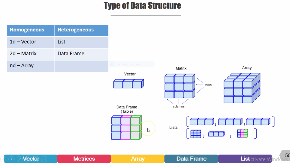
Data Structure can be defined as the specific form of organizing and storing the data. R Programming supports five basic types of data structure namely Vector, matrix, Array, , and list.
Vector:
Vector is a sequence of data elements of the same basic type. Members of a Vector are formally called components. Whenever we are storing the numerical value in ‘a’ or ‘b’ that ‘a’ or ‘b’ nothing but a Vector, so Vector is one-dimensional array used to store collection data of the same data type.
Similar kind of data type you can store like all the Numeric data(data type numeric) in a Vector, again you can store complex(data type complex) similarly in logical(data type logical) or character(data type character) you can store this thing in a Vector. There is six type of atomic Vector, they are Logical, Integer, Double, Complex, Character, and Raw.
Matrices:
Matrix is a collection of data elements of the same mode arranged in a two-dimensional rectangular layout. We can create a matrix containing only characters or only logical values, these are not of much use. We use matrices containing numeric elements to be used in mathematical calculations. They are accessed by two integer indices.
Three kinds of matrices are
Matrix Multiplication
R matrix transpose
Matrix power
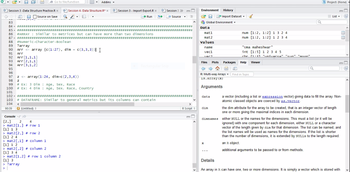
Arrays:
Similar to matrices but they can be multi-dimensional(more than two dimensions). Array function() takes vectors as input and uses the values in the dim parameter to create an array.
If you want to store age, salary, location, designation then it becomes your array. Salary or age all those things are numeric but if you store numeric as well as a character variable, character variable is nothing but a gender like male or female then you can use an array.
Data Frames:
Generalization of matrices where different columns can store in a different mode then it’s called Data Frame. It is a list of vectors of equal length. Data frame is a table or two-dimensional array like structure in which each column contains values of one variable and each row contains one set of values from each column. It can store a different kind of data types like you can store numerical with categorical and logical
Lists:
Lists are something where you can store all those other four, you can store data frame in lists, you can store an array in a list or you can store matrices and you can store a vector as well. Lists ordered a collection of objects where the elements can be of different types. Lists contain the elements of different types like-number, strings, vectors and another list inside it. Lists are created using lists function().
Types of Data Structure:
Vector, Matrix, and Array those are in the homogeneous so they can store homogeneous data either numeric, character or logical but only different in dimension, Vector is one dimension, Matrix is two dimension and Array is multidimensional.
On the other side if you talk about Data frame and lists those are in heterogeneous so they can store a different kind of data type.
VECTOR
Numeric Vector:
Now we will learn about the Vector. Suppose you want to store 42 (vec1<-42)in vector 1 then you can see the result in vector 1. Similarly if you store more than variable 1-5 (vec1<-c(1,2,3,4,5) .
Here we show you both the way either you can use combine function and use “,” and you can store 1,2,3,4,5 (vec1<-c(1,2,3,4,5) or you can store 1-5 (vec1<-c(1:5) the only advantage is suppose you want to store it 1,7,9,3,5 then also you can use the combine function and you can store it.
If you see the class of the vector 1 then it would be an integer. Likewise, if you want to access a particular suppose you have like 1,2,3,4,5 but you only access the second element of your vector then you would get probably 2 since 1-5 in store. Likewise, you can also access 1 and 3 from that vector
CharacterVector:
Within double coat, you just pass the value which you want to store. Suppose in Vec2 we want to in “universe” (vec2<-”Universe” ) but if you store more than 1 character variable.
Then you have to use the combine function (vec2<-c(“Universe”,”sun”,”moon”) and if you see the class of it then you definitely get the class as character.
If you mix the character and numeric then all the values will be converted to character.
Logical Vector:
You can store TRUE and FAlSE for the logical function. Suppose we are using vector 3. Here you store FALSE for vec3(Vec3<-FALSE). In vec3 if you store more than one variable which is TRUE and FALSE (Vec3<-c(TRUE, FALSE) and finally if you class of it, it would be logical.
If you mix the logical vector function with numeric vector function then the numeric function gets the preferences and If you mix character with logical function and numeric function then all value converted to character function so character is given the preferences.
Matrices:
Matrices are the R object, which is a collection of data elements arranged in a two-dimensional data array.Although we can create a matrix containing only characters or only logic values which are not of much use. We use matrices containing numeric elements to be used in mathematical calculations.
Matrix is created using the matrix() function.Matrix() function is being used to create a matrix. Here we show an argument.
Here,the argument is matrix(data=NA,nrow=1,ncol=1,byrow=FALSE,dimnames=NULL). We have a data, word data which we want to create a matrix, suppose 1-4 we want to create a matrix. Then, how many rows here, there are by default 1 row but we are changing it two and by default it’s column is 1 but we are also changing this to two and suppose by default byrow is equal to False and by row is nothing but suppose 1-4 you want to create a matrix then how you want to do it? Either this way byrow equal to TRUE equal to 1,2,3 and 4.
But if you change that byrow equal to FALSE then you want to do it by column so first 1 then 2 then 3 then 4 that’s how you can do it. Here, we are keeping all the numerical values but here we are showing it 2 rows and 2 columns and by rows equal to TRUE that means we will start from the row and then in the second row. Similarly, if you access any element of a matrix.
Suppose, we are creating matrix 2 where we access the first row then you can say 1,so this is row, column so we are asking for the first row and it would give us first row, the second row then it also gave us first column because we said row, column then second column.
We haven’t written anything in a row that’s why it would give us all the rows and only it would give us first column. Similarly, it would give us all the rows but an only second column.
Array:
Now we have discussed the Array. An Array is similar to matrices but it can have more than two dimensions. Here, you can store 2*3*4 anything you can create. R Array is the data objects which can store data in more than two dimensions. An Array is created using the Array() function. The array can store only data type. Array takes vectors as input and uses the values in the dim parameter to create an Array.
It can contain multidimensional rectangular shaped data storage structure. “Rectangular” in the word, each row is having the same length similarly for each column and other dimensions. But Array can store only values which have similar kind of data,i.e. variables/elements having a similar data type.We create Array using the Array() function. The argument is array (data=NA, dim=Length(data), dimnames=NULL).
We first pass the data here we pass 1 to 27 with this dataset we want to create the Array. What is those dimension? The dimension is 3*3*3 here you can store salary, age, designation, grade or something like that. It is pretty simple and you can see the result as well.
Dataframe:
Dataframe is a table or two-dimensional array like structure where each column contains values of one variable and each row contains one set of values from each column.
Data frame is used for storing a data tables. This is a list of vectors of equal length. All the vectors we have learned previously like Numerical vectors, Character Vectors, Logical Vectors and all those things. Now you just mix them the three vectors you mix them. Suppose you want to create a data frame where you have one attribute as Numerical like age or salary which is numerical but you have three employees so all of this vector like the same length. So you have three employees then you want to store their gender as well male, female. Similarly, you want to understand whether they left the company or not something like that TRUE FALSE or something like that. If you achieve this kind of data set then you have to use data frame.
Now we use data. frame, we use this data. frame function. Before that we have to three vectors first, suppose we are storing 2,3,5 a vector called num then “aa”,”bb”,”cc” in char and then TRUE, FALSE and TRUE in logical then ultimately using data.frame()function and creating that data frame. Here we are using the data frame name df. If you want to see what is df? Or what is being stored in df? Thereafter you get the result.
Think about a business scenario, where you have a lot of employees and here you use the data frame. That’s why data frame is one of the most important structures in R. In R we have a lot of inbuilt data frame which you can explore. One of the popular dataframe is mtcars. Mtcars is a dataset of a car distribution. We have df which is already been created in R that’s why we said this inbuilt database. Here mtcars has 32 model of cars. If you want to see a couple of them then you use head() function, you can use the head() function for first several rows. similarly, you can use tail() function to see last couple rows. The tail function gives you the below of the lists. Another function is str() function which is the structure of a dataset. The str() function gives you the detail observation. For str() function you get a sense how your data set looks like. Likewise, you can see the summary which is better than the full data structure. The summary() function gives you the min or max from each of those attributes.
Accessing Column from data frame:
Accessing Column from data frame is quite easy. Once you write any data frame and after that if you put “dollar sign ($)” then you would see all the columns whatever it contains and you can see whatever is there in that column.
Now, there is another way to do it, if you use “third bracket[]” and if you use row, column as I discussed earlier.
Similarly, you can name the column and you can see the column as well. But it has a problem if you have more than one column then how do you do that? In that case, you use combine function and give the number of all those columns and you can see those columns as well.
Accessing Row:
Similarly, Accessing Row is also easy. As said use third bracket and between third bracket row, column.
For an example: df[2,]
Here row value is 2 and all column value is NULL. The function is used for accessing the second row.
Dropping column:
If you want to drop a column then you don’t want the column to be included in your data frame.You simply put (-sign) before that number. If you say that you don’t want to see drop third column which is actually displacement column.
For an example: df[,-3]
df[,-c(2,3)]
So if you say within third bracket all the rows,-3 then it would actually drop that column. Similarly, if you drop second and third then it would actually drop displacement and cylinder.
Subset:
The fourth one is a subset. So, what if you don’t want to see all the rows of that column. You want to see only those observation or those car brands where the cylinder value is more than 6 or the horsepower is more than 50.
For an instance: car 1<-subset (df,cyl>6)
car 2<-subset (df,hp>50)
Then you create new data frame called car 1 using the subset function so in subset function you passing the data when you are passing the condition. Based on that your car is created, you can see it cylinder column of car data frame, has the only cylinder which is more than 6. Similarly, for horsepower also you can see the result.
If you have two data frame, so you have data frame one and data frame two now you have combined them by row. Suppose, in the first data frame you have twenty car brands and second data frame you have twelve car brands. Now you want to combine this two rbind () function.
Likewise, if you have two columns. Suppose all the 32 car brands you have the mileage which is a column and you have another one may be a cylinder. So you want to combine this column that also you can do using cbind() function.
Factor:
In a data frame, character vectors are automatically converted into factors, and the number of levels can be determined as the number of different values in such a vector. You can create a data frame using more than one data types. It can be a mixture of numeric, with a character with logical all those things.
Similarly, if you see the showing data frame which has three vectors like name, age and gender and you have created a new data frame using data.frame() function. If you see the class of it, you would get it as data.frame. But surprisingly if you see the class of name this data frame dollar could give all those names. If you see the class of it you would be surprised this is now not a character variable rather it’s now a factor. So it is another new data type.
Factor:
In a data frame, character variables are automatically changed or converted into factor, and the number of levels can be determined as the number of different values in such a vector.
Factor takes a limited number of different values, such variables are referred to as categorical variables. So, Factor represents the categorical data, the factor can be ordered or unordered and are an important class for statistical analysis and for plotting. Factor variables are very useful to many different types of graphics.
Storing data factors insures that the modeling functions will treat such data correctly. The factor can store both integers and strings. These are very useful in the columns which have a limited number of unique values such as “Male, Female” and “True, False” etc.
Factors in R has two varieties
ordered
unordered.
Factors are stored as a vector of integer values, with a corresponding set of character values to use when the factor is shown. factor() function is used to create a factor. The required argument to factor is a vector of values, which will be returned as a vector of factor values. Numeric and Character variables both can be made into factors, but a factor’s levels will always be character values.
Factor levels
Getting a dataset you will look that it contains factors with specific factor levels. By the way, sometimes you will willing to change the names of these levels for clarity or any other reasons. R permits you to do this with the function levels().
Examples:
for this is mtcars data:
>Str (mtcars)
$ cyl : num 6 6 4 6 8 6 8 4 4 6
Here, have shown an example, suppose this is mtcars data where has 32 car brands. Each of those cars we have eleven attributes like horsepower, cylinder, displacement, mileage or all those things. If you see the cylinder, either it has 6 as cylinder or 4 as cylinder or 8 as a cylinder. So, since if you have a minimum number of unique value of particular attributes then that’s an ideal candidate for factors. Because it does not take 6.5 or 4.32 or 5.67. It takes either 4 or 6 or 8 so we want to change this to a factor.
Str (mtcars)
mtcars$cyl = as.factor(mtcars$cyl)
How to use factor() function? Just use as.factor() function, here the first query is which one you want to change? Suppose, here change the “mtcars$cylinder”.You can access it any column using the dollar function. Using that “as.factor()” function,the “mtcars$cylinder” is converting into Factor.
Str (mtcars)
$ cyl : num 6 6 4 6 8 6 8 4 4 6
Now, looking carefully at the above example, look the structure of “mtcars” when it changes to factor then everything is changed into the numeric function. Changing this when you look at the cylinder, it is converted to a factor. After changing it has three level 4,6 and 8.
str (mtcars)
(four column or four attributes change to numericals factors)
If it is changed whether manually or automatically. What is the number of gear of the mtcars or how many numbers of carburetors is there, then you see the number of the structure of mtcars. Now you see all those columns or all those attributes as change into factor. You can notice that automation has two levels if it is manual or automatic.
str (mtcars)
(four column or four attributes change to numericals factors)
Similarly, you have 6 levels of carbs. That’s how you can change it.
How to change the name of the level?
If you change the name of the level, then you have to create a new variable called gender vector and then you want to store “Male”, “Female” , “Female” , “Male” , “Male”. It may be a data for five employees. Thereafter, you see that the five things have been recorded. If you see the class of gender vector then it is a character vector.
But, if you want to change the gender vector to factor
#Convert gender vector to factor
factor-gender-vector <-as.factor(gender vector)
factor-gender-vector # factor gender has two levels Male and Female
then use “as.factor” and then see it has changed to a factor and it’s showing the level is “Female Male”.
Now you want to change the name of the factors using level()
levels(factor-gender-vector)<-c(“f” , “M”)
levels: Female and Male(earlier)
Now, it changes to “F & M”
That’s how you want to do it.
How to do that? In this case, level() function helps you. Using level() function which you want to change, just give this. Suppose you want to change “factor-gender and vector”. Here suppose you want to change F and M for Female and Male. once you can do it and you can again see this, this levels have changed. Previously it showed Female and Male now it changes to F and M. in this process you want to do it.
List:
These are the most complex data structure. A List may contain a combination of vectors, matrices, data frames and even other list itself. The list is being created using List() function in R. A list is a generic vector containing other objects. Lists is a data structure containing of mixed data types. A vector which have all elements of same type is called atomic vector but a vector having elements of various type is called List.
Before creating a list, creating a vector suppose you create a vector with one to ten(1-10).
Thereafter you create a matrix which is two dimensional array.
Then you will create a data frame, that is “mtcars” which was inbuilt data frame but here you just take only three observation and create a data frame called “my-dataframe” from “mtcars”.
Finally, you will store this vector, matrix and dataframe in a list called “my list”, using the list() function.
If you created the list() then you see the result. You can see the output from “mylist”. Here the list starts from the first vector,”my-vector” is one to ten.
Creating list:
# vector with numerics from 1 up to 10
>my-vector <-1:10
The output is
[[1]]
Thereafter you create a matrix which is two dimensional array that “my-matrix”.
# matrix with numerics from 1 up to 9
>my-matrix <-matrix(1:9,ncol =3)
The output is
[[2]]
Then you just created the data frame
# first 3 rows of the built in data frame “mtcars”
>my-df <-mtcars [1:3,]
The result is
[[3]]
That’s the way to do a list.
If you see these examples there's no name like [1], [2], and [3] is written of the list but you can change those name as well using the name() function.
#give name using name()
>names (my list)<-c (“vec”, ”mat”, ”df”)
Then you can check the output and see the name would be changed.
How does a list() work?
At first you create vector() function
my-vector<-1:10
Then use matrix function
my- matrix<-(matrix 1:9, ncol=3)
Thereafter creating a dataframe
my-df<-mtcars[1:3,]
Here”mtcars” is the data where you can see all those 32 car brands and eleven attributes but the first 3 rows uses for this dataframe.
Then using the list() function,created a list
my-list < - list(my-vector,my-matrix,my-df)
Then the output is my-matrix ,my-vector, and my-df
1.
2.
3.
In this way list works.
List is the end of data structure. Any character variables when it goes to data frame it automatically changes to a factor but if you don’t want to do this then you can change that things from anything to anything. Here show you how to change anything to a factor using as.factor but later you also know where you will be change it to,as numeric() function or as character() function. mutate(),filter(),arrange() Function
Selecting columns using select()
select() keeps only the variables you mention
Use This Command To Perform The Above Mentioned Function
####################################### #select(): Select specific column from tbl ####################################### tbl <- select (hflights, ActualElapsedTime, AirTime, ArrDelay, DepDelay ) glimpse(tbl)
#starts_with("X"): every name that starts with "X", #ends_with("X"): every name that ends with "X", #contains("X"): every name that contains "X", #matches("X"): every name that matches "X", where "X" can be a regular expression, #num_range("x", 1:5): the variables named x01, x02, x03, x04 and x05, #one_of(x): every name that appears in x, which should be a character vector.
#Example: print out only the UniqueCarrier, FlightNum, TailNum, Cancelled, and CancellationCode columns of hflights
mutate() is the second of five data manipulation functions you will get familiar with in this course. mutate() creates new columns which are added to a copy of the dataset.
Use This Command To Perform The Above Mentioned Function
####################################### #mutate(): Add columns from existing data ####################################### g2 <- mutate(hflights, loss = ArrDelay - DepDelay) g2
Filtering data is one of the very basic operation when you work with data. You want to remove a part of the data that is invalid or simply you’re not interested in. Or, you want to zero in on a particular part of the data you want to know more about. Of course, dplyr has ’filter()’ function to do such filtering, but there is even more. With dplyr you can do the kind of filtering, which could be hard to perform or complicated to construct with tools like SQL and traditional BI tools, in such a simple and more intuitive way.
R comes with a set of logical operators that you can use inside filter(): • < • <= • == • != • != • >
Use This Command To Perform The Above Mentioned Function
#filter() : Filter specific rows which matches the logical condition ####################################### #R comes with a set of logical operators that you can use inside filter():
#x < y, TRUE if x is less than y #x <= y, TRUE if x is less than or equal to y #x == y, TRUE if x equals y #x != y, TRUE if x does not equal y #x >= y, TRUE if x is greater than or equal to y #x > y, TRUE if x is greater than y #x %in% c(a, b, c), TRUE if x is in the vector c(a, b, c)
# All flights that traveled 3000 miles or more long_flight <- filter(hflights, Distance >= 3000) View(long_flight) glimpse(long_flight)
# All flights where taxing took longer than flying long_journey <- filter(hflights, TaxiIn + TaxiOut > AirTime) View(long_journey)
# All flights that departed before 5am or arrived after 10pm All_Day_Journey <- filter(hflights, DepTime < 500 | ArrTime > 2200)
# All flights that departed late but arrived ahead of schedule Early_Flight <- filter(hflights, DepDelay > 0, ArrDelay < 0) glimpse(Early_Flight)
# All flights that were cancelled after being delayed Cancelled_Delay <- filter(hflights, Cancelled == 1, DepDelay > 0)
#How many weekend flights flew a distance of more than 1000 miles but #had a total taxiing time below 15 minutes?
To arrange (or re-order) rows by a particular column such as the taxonomic order, list the name of the column you want to arrange the rows
Use This Command To Perform The Above Mentioned Function
####################################### #arrange(): reorders the rows according to single or multiple variables, ####################################### dtc <- filter(hflights, Cancelled == 1, !is.na(DepDelay)) #Delay not equal to NA glimpse(dtc)
# Arrange dtc by departure delays d <- arrange(dtc, DepDelay)
# Arrange dtc so that cancellation reasons are grouped c <- arrange(dtc,CancellationCode )
#By default, arrange() arranges the rows from smallest to largest. #Rows with the smallest value of the variable will appear at the top of the data set. #You can reverse this behavior with the desc() function.
# Arrange according to carrier and decreasing departure delays des_Flight <- arrange(hflights, desc(DepDelay))
# Arrange flights by total delay (normal order). arrange(hflights, ArrDelay + DepDelay)
#######################################
The summarise() function will create summary statistics for a given column in the data frame such as finding the mean.
Use This Command To Perform The Above Mentioned Function
####################################### #summarise(): reduces each group to a single row by calculating aggregate measures. ####################################### #summarise(), follows the same syntax as mutate(), #but the resulting dataset consists of a single row instead of an entire new column in the case of mutate()
#min(x) - minimum value of vector x. #max(x) - maximum value of vector x. #mean(x) - mean value of vector x. #median(x) - median value of vector x. #quantile(x, p) - pth quantile of vector x. #sd(x) - standard deviation of vector x. #var(x) - variance of vector x. #IQR(x) - Inter Quartile Range (IQR) of vector x. #diff(range(x)) - total range of vector x.
# Print out a summary with variables # min_dist, the shortest distance flown, and max_dist, the longest distance flown summarise(hflights, max_dist = max(Distance),min_dist = min(Distance))
# Print out a summary of hflights with max_div: the longest Distance for diverted flights. # Print out a summary with variable max_div div <- filter(hflights, Diverted ==1 ) summarise(div, max_div = max(Distance))
Before we go any futher, let’s introduce the pipe operator: %>%. dplyr imports this operator from another package (magrittr). This operator allows you to pipe the output from one function to the input of another function. Instead of nesting functions (reading from the inside to the outside), the idea of of piping is to read the functions from left to right.
Use This Command To Perform The Above Mentioned Function
####################################### #Chaining function using Pipe Operators ####################################### hflights %>% filter(DepDelay>240) %>% mutate(TaxingTime = TaxiIn + TaxiOut) %>% arrange(TaxingTime)%>% select(TailNum )
# Write the 'piped' version of the English sentences. # Use dplyr functions and the pipe operator to transform the following English sentences into R code:
# Take the hflights data set and then ... # Add a variable named diff that is the result of subtracting TaxiIn from TaxiOut, and then ... # Pick all of the rows whose diff value does not equal NA, and then ... # Summarise the data set with a value named avg that is the mean diff value.
# mutate() the hflights dataset and add two variables: # RealTime: the actual elapsed time plus 100 minutes (for the overhead that flying involves) and # mph: calculated as Distance / RealTime * 60, then # filter() to keep observations that have an mph that is not NA and that is below 70, finally # summarise() the result by creating four summary variables: # n_less, the number of observations, # n_dest, the number of destinations, # min_dist, the minimum distance and # max_dist, the maximum distance.
The group_by() verb is an important function in dplyr. As we mentioned before it’s related to concept of “split-apply-combine”. We literally want to split the data frame by some variable (e.g. taxonomic order), apply a function to the individual data frames and then combine the output.
Use This Command To Perform The Above Mentioned Function
#######################################
#group_by function
#######################################
# Most data operations are done on groups defined by variables.
# group_by() takes an existing tbl and converts it into a grouped tbl where operations are performed "by group".
# Make an ordered per-carrier summary of hflights
hflights %>%
group_by(UniqueCarrier) %>%
summarise(p_canc = mean(Cancelled == 1)*100,
avg_delay = mean(ArrDelay,na.rm = TRUE))%>%
arrange(avg_delay, p_canc)
# summary of hflights without per carrier
hflights %>%
summarise(p_canc = mean(Cancelled == 1)*100,
avg_delay = mean(ArrDelay,na.rm = TRUE))%>%
arrange(avg_delay, p_canc)
# Ordered overview of average arrival delays per carrier
# mutate() uses the rank() function, that calculates within-group rankings.
# rank() takes a group of values and calculates the rank of each value within the group,
Dates can be imported from character, numeric formats using the as.Date function from the base package.
If your data were exported from Excel, they will possibly be in numeric format. Otherwise, they will most likely be stored in character format. If your dates are stored as characters, you simply need to provide as.Date with your vector of dates and the format they are currently stored in
There are a number of different formats you can specify, here are a few of them:
%Y: 4-digit year (1982)
%y: 2-digit year (82)
%m: 2-digit month (01)
%d: 2-digit day of the month (13)
%A: weekday (Wednesday)
%a: abbreviated weekday (Wed)
%B: month (January)
%b: abbreviated month (Jan)
Use This Command To Perform The Above Mentioned Function